Rolling-window returns: Brazilian equities versus the CDI, 1995 to 2019

This analysis covers data to 2019. It was written as an exploratory exercise rather than as research, and it is retained here because the method is still sound.

Summary: for almost all investment window sizes, with or without taxation, investing in an IBOV tracking security or fund performed, on average and in most cases, better than investing in Brazil’s CDI tracking government bonds (Tesouro Direto, LFT).

One of these days I overheard a colleague mentioning a Twitter debate in which, from what I understood, one person was defending that the best passive investment strategy was investing in Brazil’s fixed income bonds (which yield Brazil’s CDI fixed income rate), while the other person defended that investing in Brazil’s main stock market index (IBOV) (or in some IBOV index fund) would yield a better result.

That got me curious, so I started writing some scripts to be able to give a quantitative perspective to this debate.

The question that I tried to answer with my research was: which investment was more profitable on average for a given investment window?

To accomplish this task I wrote code that calculated the return for each index¹ for all possible window sizes. I used the data starting from 1995-01-01 to eliminate pre plano real hyper-inflation effects.

Windowing

So what is windowing anyway? Let’s say that a given security has the following daily returns:

>>> returns = [0.987, 1.01, 1.003, 1.013, 1.12, 0.98, 0.81]

This means that the value of the security on day 1 is 1.01 times the value of this security on day 0. Writing V[i] for the security’s value on the i-th day and r[i] for its return as a ratio on that day:

V[i] = V[i-1] * r[i]    which is the same as    r[i] = V[i] / V[i-1]

In our example we have 7 days of returns. If we want to know the total (cumulative) return of this security during the whole period we only need to multiply all daily returns:

>>> import numpy as np
>>> np.prod(returns)  # equivalent to returns[0] * returns[1] * ...
0.9004881914524542

Now let’s imagine that on the 3rd day we decided to sell the security. In that case the total return of our investment will be:

>>> np.prod(returns[:3])
0.9998606099999999

That’s better. But what if instead of investing on day 0 and selling on the 3rd day we invest on the first day and sell on the 4th?

>>> np.prod(returns[1:4])
1.0261993899999997

That’s much better. In this case we still invested for 3 days but instead of starting on day 0 we started on day 1. We say that in both cases our investment window was 3 days long.

Let’s continue our experiment by analysing this security’s return for each 3-day window size. As we have 7 days worth of returns we can calculate the return for the following 3-day windows:

• Start at 0, finish at 2
• Start at 1, finish at 3
• Start at 2, finish at 4
• Start at 3, finish at 5
• Start at 4, finish at 6
• Start at 5, finish at 7

This can be accomplished with the following code:

>>> for start_index in range(len(returns) - 2):
...     end_index = start_index + 3
...     text = f'Starting at {start_index}, stopping at {end_index - 1}'
...     r = np.prod(returns[start_index:start_index + 3])
...     print(f'{text}: {r}')
...
Starting at 0, stopping at 2: 0.9998606099999999
Starting at 1, stopping at 3: 1.0261993899999997
Starting at 2, stopping at 4: 1.1379636799999997
Starting at 3, stopping at 5: 1.1118688
Starting at 4, stopping at 6: 0.8890560000000002

We can also estimate what the returns would be for each window size:

>>> for window_size in range(1, len(returns) + 1):
...     for start_index in range(len(returns) - (window_size - 1)):
...         end_index = start_index + window_size
...         text = f'Window size: {window_size}, starting at {start_index},' \
...                f' stopping at {end_index - 1}.'
...         r = np.prod(returns[start_index:start_index + 3])
...         print(f'{text}: {r}')
...
Window size: 1, starting at 0, stopping at 0.: 0.9998606099999999
Window size: 1, starting at 1, stopping at 1.: 1.0261993899999997
Window size: 1, starting at 2, stopping at 2.: 1.1379636799999997
Window size: 1, starting at 3, stopping at 3.: 1.1118688
Window size: 1, starting at 4, stopping at 4.: 0.8890560000000002
Window size: 1, starting at 5, stopping at 5.: 0.7938000000000001
Window size: 1, starting at 6, stopping at 6.: 0.81
Window size: 2, starting at 0, stopping at 1.: 0.9998606099999999
Window size: 2, starting at 1, stopping at 2.: 1.0261993899999997
Window size: 2, starting at 2, stopping at 3.: 1.1379636799999997
# ...
Window size: 4, starting at 2, stopping at 5.: 1.1379636799999997
Window size: 4, starting at 3, stopping at 6.: 1.1118688
Window size: 5, starting at 0, stopping at 4.: 0.9998606099999999
Window size: 5, starting at 1, stopping at 5.: 1.0261993899999997
Window size: 5, starting at 2, stopping at 6.: 1.1379636799999997
Window size: 6, starting at 0, stopping at 5.: 0.9998606099999999
Window size: 6, starting at 1, stopping at 6.: 1.0261993899999997
Window size: 7, starting at 0, stopping at 6.: 0.9998606099999999

You have just seen exactly what I am doing with the CDI’s and IBOV’s returns: I calculated the return for each window size for every possible starting day (notice that the number of possible windows in the period decreases as the window size increases).

In all of this post’s graphs the horizontal axis represents a window size (usually in years) and the vertical axis the total (cumulative) return.

The data

Some data was scraped and downloaded, and some was generated from the original data.

Data sources

• CDI data: Calculadora do Cidadão, Banco Central do Brasil
• IBOV data: Comdinheiro

The results

Let’s start by taking a look at the quartile distribution of the CDI and IBOV indices:

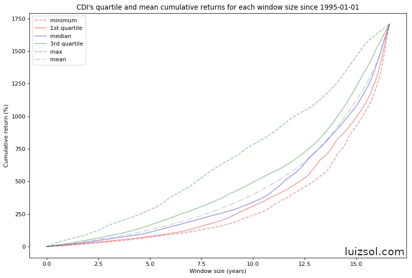
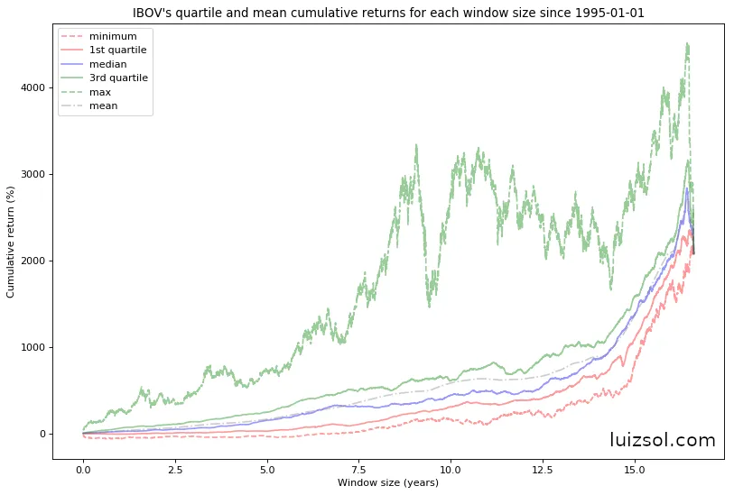
As we can see in the figures above, as expected the IBOV returns are much more positively skewed than the CDI returns for almost all investment windows, which is a direct consequence of the higher IBOV volatility.

Now, even though it gives us no further knowledge about the data, let’s plot all IBOV and CDI percentiles for all windows:

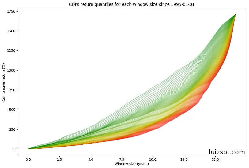
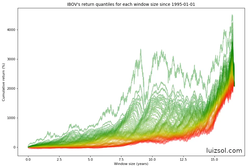
The graphs above show all return percentiles (from 0 to 100), transitioning from 0 = red to 100 = green.

If we do a semi-log plot of both graphs, in order to reduce the effect of the scale of bigger windows, we get the following:

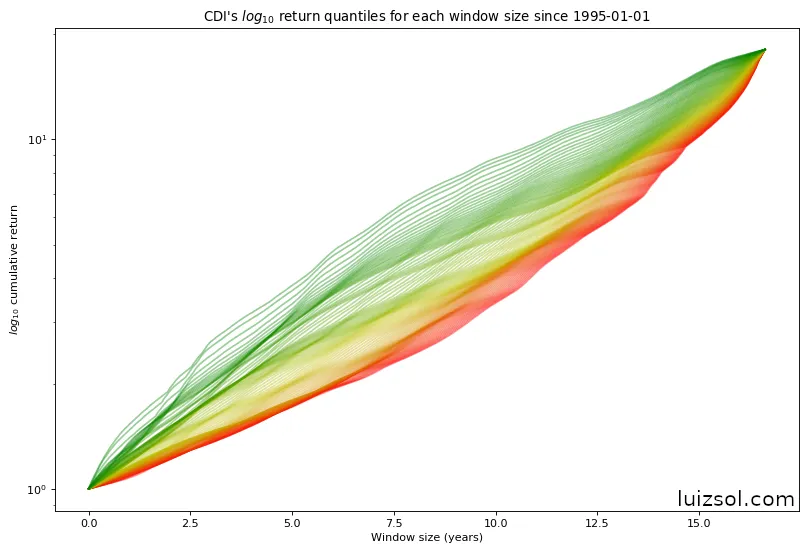
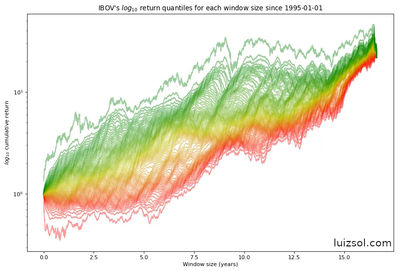
Quick refresher on reading those vertical axes, where r is the cumulative return as a ratio:

• log10(r) = 0.1 means a profit of 12.58% minus 100%, so -87.41%
• log10(r) = 1 means a profit of 100% minus 100%, so 0%
• log10(r) = 2 means a profit of 1000% minus 100%, so 900%

Taking a look at the after-tax² percentiles:

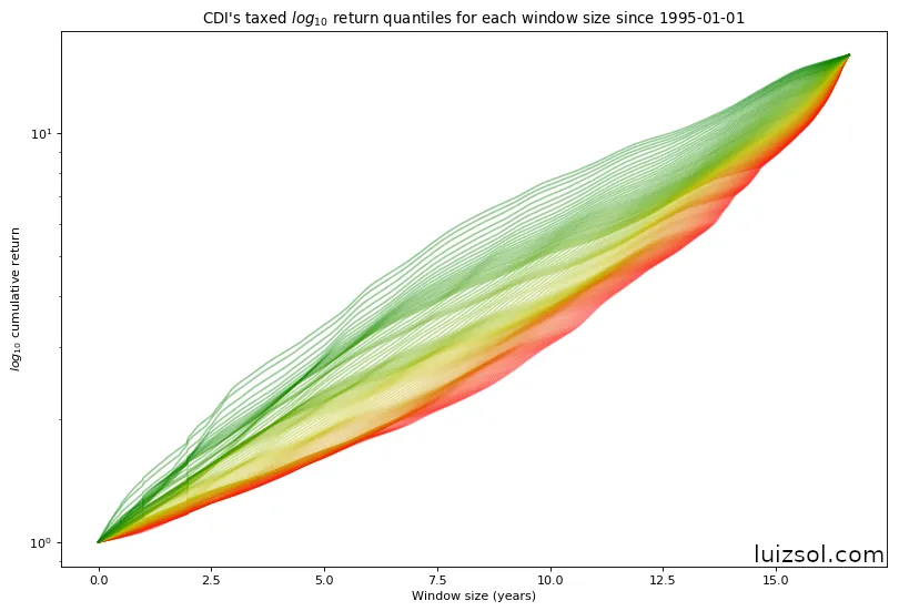
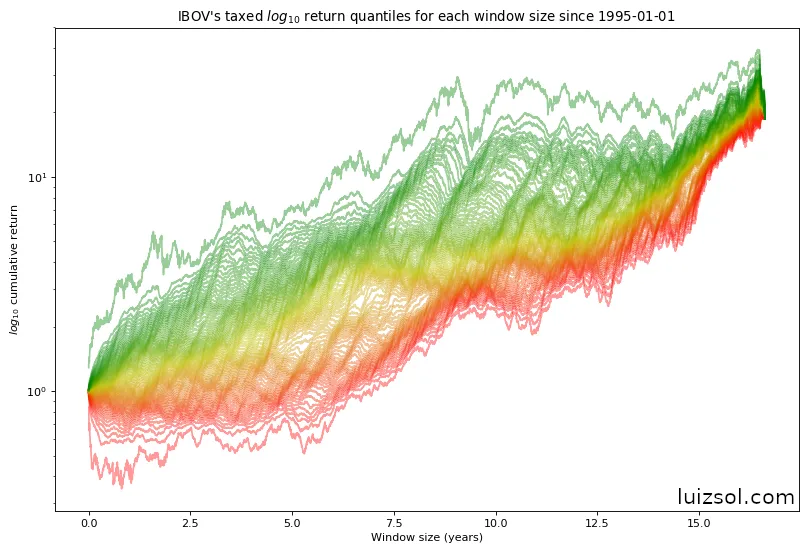
Now that we have a good idea of the distribution of returns for each window size for each index let’s compare them. Let’s first start by comparing their averages:

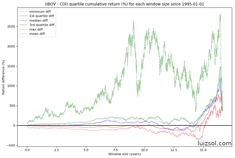
This graph shows us that, for almost all window sizes, both on average³ (the difference between the average window returns is positive) and in most cases⁴ (the difference between the median window returns is positive) it was better to invest in an IBOV indexed security than in a CDI indexed one.

Let’s now take a look at the difference between all window quantiles, both pre and post tax:

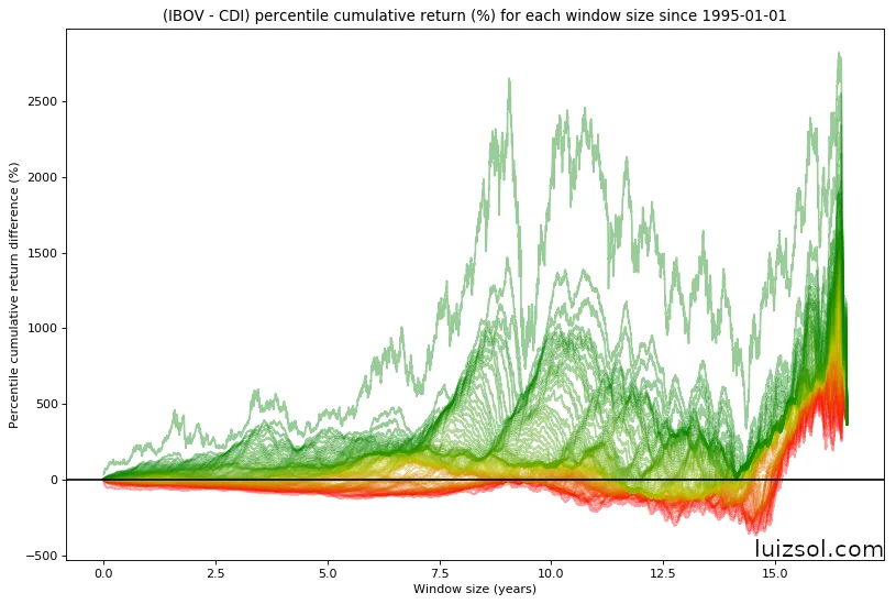
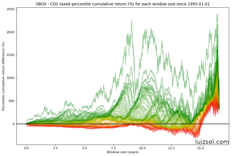
Looking at this graph we get the strong impression that, almost always, IBOV was a better passive investment than CDI over this period.

Take a look at the graphs below:

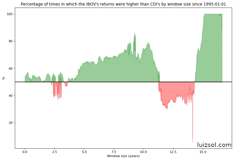
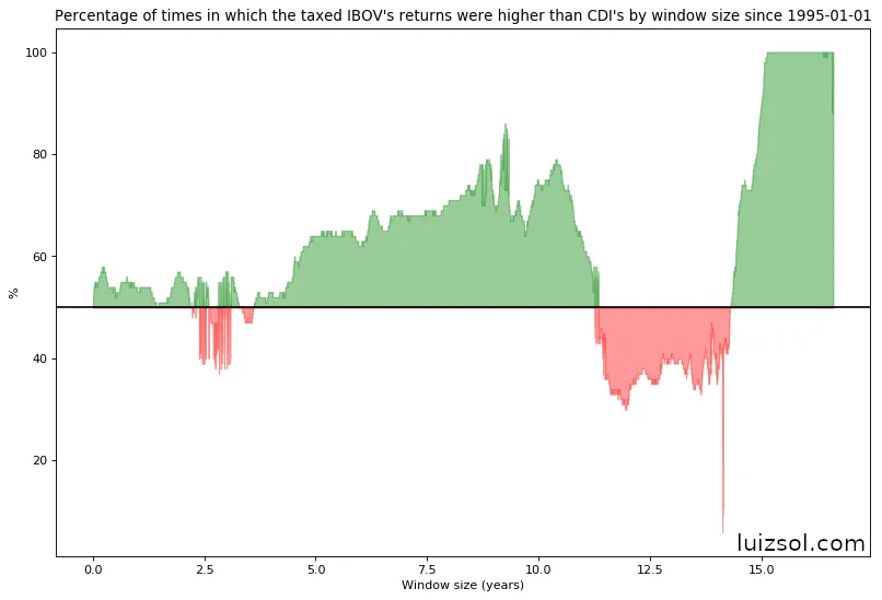
The line in the graphs above represents, for each window size, the proportion of windows in which the IBOV return was greater than that of the CDI.

A simple interpretation of the graphs above is the following: imagine that we go back in the past and pick, at random, a day to start investing in both CDI and IBOV indexed securities. The line represents, for each window size, the proportion of cases in which the IBOV indexed security performed better than the CDI indexed security.

I drew a line in the middle of the graphs so we can see the window sizes for which an IBOV indexed security outperformed a CDI indexed security in most cases.

Conclusion

Over the period covered, and on this method, an IBOV indexed security outperformed a CDI indexed security in most windows of most sizes, both before and after tax. That is a description of what happened between 1995 and 2019, not a prediction and not a recommendation.

It is also quite interesting to see that for investment windows between 11 and 14 years it was better to have invested in CDI than in IBOV.

My impression

I have to admit that I am pretty impressed. Brazil is notorious for its historically high government bond interest rates, so I always believed that CDI indexed securities would beat Brazil’s main stock market, especially over big investment windows. It is always good to know when you are wrong.